Euler-Lagrange Equation - why is it so useful? (Part 2/2)

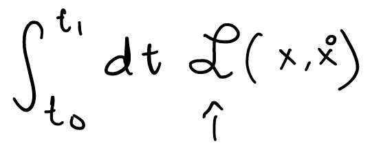
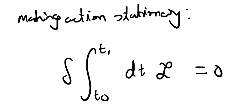
In my last post I mentioned two main advantages of this equation in the world of physics and particularly the modelling of the law of motion. In this post, I'm going to delve a bit deeper on both these advantages. And for those of you who think I've gone crazy about this one particular mathematical equation, don't worry! I have something in store for all of you in the next post (hint: everything we are doing here can be used to calculate stuff about the orbit of the Earth, our solar system, our galaxy and really our whole universe). So yeah, pretty important stuff here.

Let's dive in:

1. Its form is essentially the same in any coordinate system. This means you can switch between cartesian, polar and other coordinate systems with multiple variables seamlessly using this equation. Trying to apply Newtonian equations in these different systems would be tedious without this 'translator'. In particular, this equation implicitly encompasses the basic laws of physics.

So, this is probably the hardest to prove. But here's my attempt at it.

Let's prove this by looking at a conversion between two coordinate systems that most of you have probable heard of: cartesian and polar. For those of you who may need a refresher, the cartesian coordinate system is our usual x-y coordinates. The polar system defines coordinates by taking their distance from the origin and the angle made by this point. Here's a simple polar coordinate system:

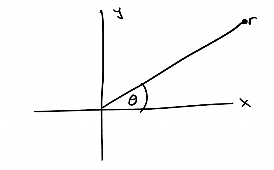
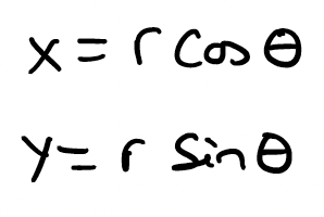
Theta represents the angle that we measure. Coordinates in this system are derived using the following equalities:

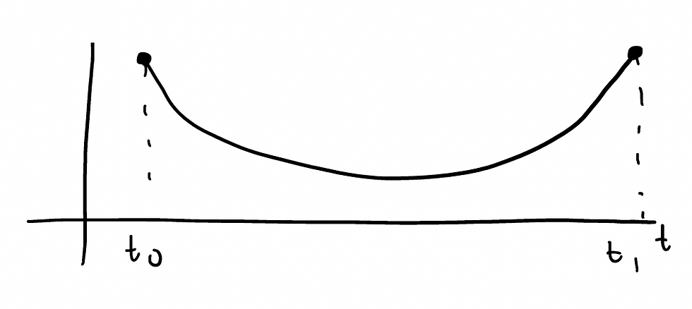
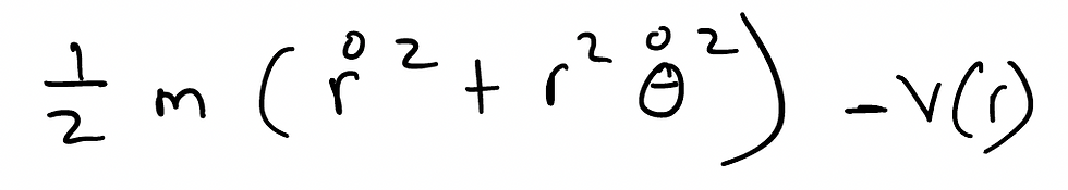
Now, let's define our Lagrangian as the Kinetic Energy (KE) minus the Potential Energy (PE). This is quite conventional, as this represents the total energy existing in a system (remember that total energy consists of both kinetic and potential energy). Let's define our Lagrangian in such a manner:

In this, V(X) represents the potential energy and the second formula is for the kinetic energy. From elementary physics, we know the formula of KE to be 1/2*mv^2 where m stands for mass and v stands for velocity. Anyone who has read my notes on introductory cosmology will know that an open circle over a variable represents the time derivative of that variable. Since x has represented position in my notes, an open circle over x is the time derivative of position, which is velocity. Both these energies make up our Lagrangian.

Let's adapt this a little bit to fit our polar coordinate plane. The PE will remain the same, except instead of having x as the position of our particle, we now have r. This is because the radius represents the position of a particle as it makes its way through the system in a polar plane (it's one of the underlying mechanisms of a polar coordinate system). The KE will change a bit. The velocity is now dependant on both x and y, since they both represent the position of the particle, which in turn impacts the velocities. So our velocity is now a sum of our individual time derivatives of x and y. As such, our kinetic energy formula can be defined as:

And replacing the x and y with our polar equivalents, we get the following result for our Lagrangian:

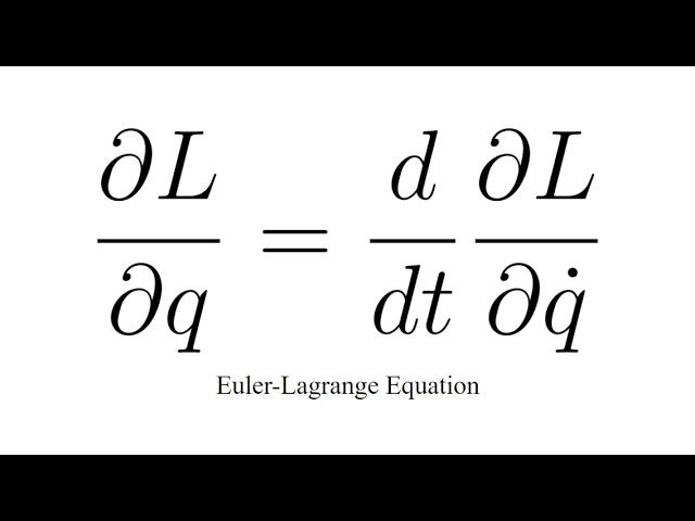
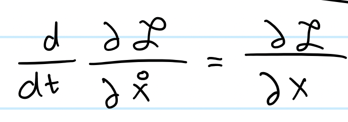
We've got our Lagrangian and we're now ready to go. Let's revisit the Euler-Lagrange Equation (E-L-E):

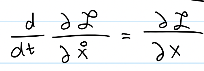
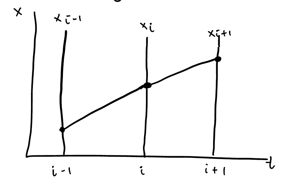
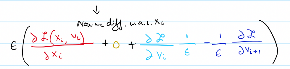
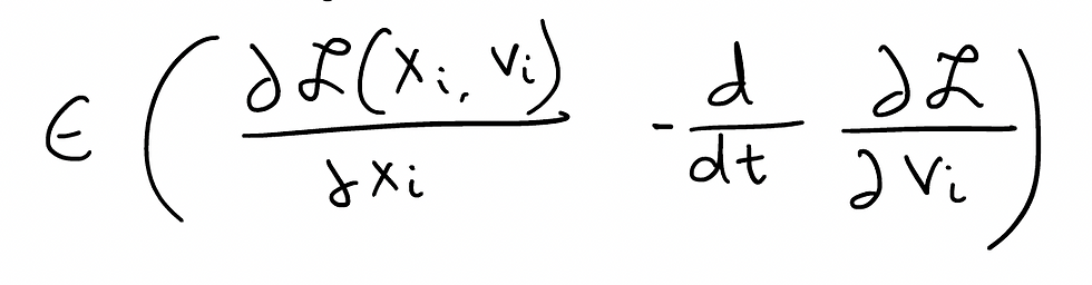
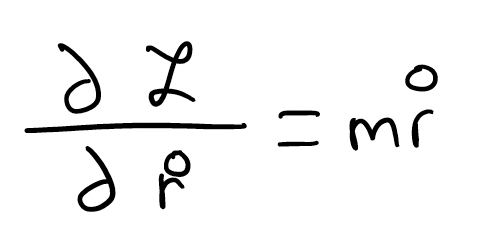
I'm going to focus on the left-hand side first. It tells me that I should first take a partial derivative of the Lagrangian with respect to the velocity.

Next, I'm going to differentiate this with respect to time:

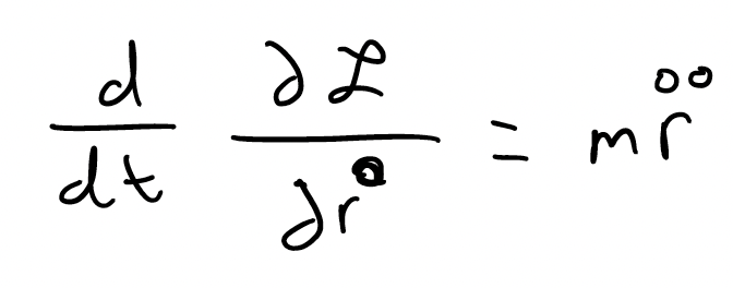
I'm now going to equate this to the right hand side of the ELE. The RHS dictates that I take a partial derivative of the Lagrangian with respect to the position and by doing so, I get:

And so, the answer to this is as simple as solving a differential equation. Using its solution, you would be able to solve problems within the laws of motion and physics. In such a way, the ELE can help converting between coordinate systems quite simply. We replaced the x-y cartesian coordinates with their polar counterparts. This might seem a bit complex, and that's because it is. It's not simple mathematics and I've presented a rather rudimentary version of a coordinate change using the powerful equation that we derived in the previous post. I'll link some videos and books that I believe describe this equation in greater detail. But for now, I'll move on to the next point.

2. A fascinating solution to a part of this equation can reveal whether there is a conservation law.

Let's pick up where we left off in the previous section. We are now going to explore the characteristics of theta. And to find these, instead of taking the partial derivative of the Lagrangian with respect to velocity, let's take it with respect to theta. Doing this, we get a peculiar solution:

Look familiar? Don't worry if it doesn't, it's the formula for angular momentum. And one trait of angular momentum is that it does not change along with time, in that it's not directly affected by time as a variable. So following the LHS of the ELE, we get:

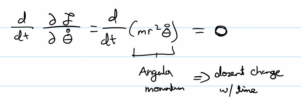
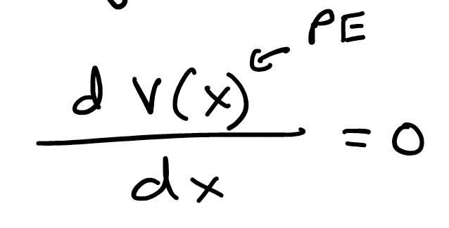
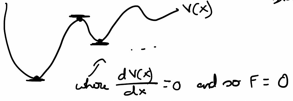
And so, we have successfully uncovered a fascinating result. If we take the time derivative of the partial of a Lagrangian, and the result is zero, we can say that the quantity is conserved. In this scenario, we say that the angular momentum is conserved.

In general, if a Lagrangian does not have a particular coordinate (in this case, it wasn't dependant on time) then the time derivative of it will be equal to 0 and we can identify it as a conservation law.

And in such a manner, we've proven two important characteristics of the ELE. While the first is insanely useful which conducting any activity in classical physics, I cannot stress how impactful the second application of the ELE is. In fact, in my next post, I'm going to compile all this information into a general, non-mathematical context and talk about what exactly does all of this imply in our world - the real world. And trust me, it implies a lot.

Till then, take some time to digest this information. I'm not an expert on any of this but rather just a student. It took me quite some time to wrap my head around many aspects of these applications of the ELE and if it's the same for you definitely reach out and I'll try and explain it in a simpler manner. See you soon!

Euler-Lagrange Equation - what is it? (Part 1/2)

Anyone who's taken a slightly rigorous calculus course or learnt anything about differential equations knows the two names I've mentioned in the title. But perhaps you aren't aware about the equation or what it means.

Well, I've got this post to explain just that and answer these questions. But firstly, let me start off by stating why exactly this particular equation is important. A vital part of classical mechanics, the Euler-Lagrange equation is used a lot for optimisation problems. It's used mainly due to 2 large advantages:

1. Its form is essentially the same in any coordinate system. This means you can switch between cartesian, polar and other coordinate systems with multiple variables seamlessly using this equation. Trying to apply Newtonian equations in these different systems would be tedious without this 'translator'. In particular, this equation implicitly encompasses the basic laws of physics.

2. A fascinating solution to a part of this equation can reveal whether there is a conservation law.

I'll go over both of these in detail, although not all in one post, since that might get a bit too dense and boring. In this post I'm going to derive the actual equation and I'll go over its implications and advantages in my future posts. One big piece of feedback I received on my previous post was the lack of explanation and clarity in my notes. Taking some of this criticism in, I've decided to give a guided tour through my notes on this topic. Hopefully by the end of this post, most of you will walk away knowing more about this extremely useful and fascinating equation.

Before starting, I'd also like to mention that there are many approaches by which you can derive this equation. The approach I've used is a bit different from ones you might find in youtube videos. I've done this through my readings of Leonard Susskind's famous book "Classical Mechanics: The Theoretical Minimum". They're a great series of books from a great physicist.

So, let's get started. I'm gonna start with something very basic. Let's take two points:

How would you go from one point, the one on the left say, to the point on the right? Well, there are many routes you could take. One of the routes (and the fastest one) is a straight line. But you could also have wacky curves all around the page that then circle back to the point. But in a system consisting of these two points (let's think of the points as particles), when is the system stationary? in other words, when is this system at rest?

Well naturally, if we want a system to be a rest, the first assumption we make is that the net force in this system is 0 (F=0). Now, and this is key, we borrow from basic laws of physics and energy conservation. In these set of laws, it states that force (F) can be described as derivatives of potential energy (PE). So, if F=0 then:

From elementary calculus, we know that if the derivative of a function is 0, it describes minima, maxima or saddle points. Here's an illustration as a reminder:

We're looking at all of this as a particle, stationary in space, but what if the particle is moving (as it most often is)? How do you calculate stationarity then?

To solve this, let's first define a movement in x (position) by delta-x:

Our new equilibrium is when delta-v = 0, or when the potential energy does not move even as the particle does. This is going to be a new general law of equilibrium (or rather, of stationarity). If a particle is moving though, we are not very interested in different points where it existed (let's not get into their existence and probabilities waves - it's an exciting topic and one that I intend to cover in future posts but for now, lets stick to non-quantum mechanisms). Rather, we are more interested in the trajectory of the particle. If the existence of a particle is shown through a point in a coordinate system, the trajectory is naturally shown through functions. So now, we do the same things we did above, but now with functions.

Coming back to my original point, take the two points in the coordinate system I asked you about at the very beginning. Let's join these two points through a wavy curve:

I'm going to take two arbitrary points within this curve and try and find the trajectory of a particle running through these points (which are in yellow). Using Pythagoras' theorem, we derive the following equation:

After some boring algebra, we arrive at the following equation for s (the total distance between the two points). All I did in between these two steps is take a dx out of the square root and then integrate both sides to find s:

If s is the distance between the two points, minimising this will give us the shortest distance between the two points. Trying to find this, we venture further and get to this step:

Seems familiar right? Well, just take that whole integral term and replace it with v and its exactly what we had in our equilibrium condition earlier! Pretty neat, right?

This solution can be proven in any coordinate system. If you take two points on the surface of the Earth, you would still get the same equation, just a bit different because the shortest distance between the two points is no longer a straight line. But I'm not going to take up your time in this post any longer, I'll get to the point now.

Let's take a different coordinate system - one with time (t) and position (x) which is dependant on time. Take two points on the graph again and connect it with a curve.

Trying to find stationary points between these two time intervals, we use what we got before. Instead of dx, we now have dt. And instead of the whole square-root term, we have what we call the Lagrangian.

Hmm, that's surprising. Why is the Lagrangian a function of both position and velocity? Easy, distance speed and time have a relationship together.

If we wanted to make this stationary, we use our general equilibrium rule:

That seems complicated and difficult. Let's make it simpler by reducing it. This first thing to do is to divide the time interval into equal increments (factor of epsilon). Next, let's divide the trajectory into these division. Here is the result:

I've labelled 3 time increments on the graph: timepoints i-1, i and i+1. Calling back to an early integration class, we are going to do something very similar to Reimann sums. Instead of depicting the integral of dt, we are instead going to express this using summations. Specifically, if we focus in on the chosen time interval, we sum the Lagrangian over the time interval (i) to obtain the following equality:

The key to understanding this step is to understand the meaning of integral, which is really to find the areas underneath the graph. By summing these individual areas, we are obtaining essentially the same result.

To make this even simpler, let's only focus on the i time interval. Here's the graph above zoomed in:

From this, we have two terms, one for the distance between i-1 and i and one for the distance between i and i+1. Remember, we no longer have integrals but rather summations.

I've colour coded each term in a different colour. This is useful for our next step. We will now do exactly the same thing we did previously to find the equilibrium. We want to find where the derivative of this is 0. Taking the derivative of this term with respect to xi, we get:

Or, simplified:

So, after all of that, we get:

Or, to put it in a different way:

And voila! What you see above is the general form of the Euler-Lagrange equation.

In the second post, I'll go over how we derive Newtonian equations from this equation, how we can work in different coordinate planes seamlessly and how we can spot a conservation law. These topics are a bit more complex, but I'll try and break it down into simpler parts as much as possible!

I hope you enjoy this post! If you liked it, leave me a message! See you all soon!

What Newton did (and what he didn't do) - my notes on the principles of cosmology

The past few posts on this blog got a little bit off topic (I think at least). For a blog that's meant to be focused on astrophysics, it didn't really have much physics in it. So this week I decided to shift gears a little bit.

Here is not a blog post but rather an introduction towards a 2 part set of notes. These notes cover fundamentals from the principles of cosmology: Newtonian equations, Friedmann equations and finding a constant for the rate of expansion of the universe. All these derivations eventually lead to a model for the expansion of the universe over time.

These notes are heavily inspired and guided by the lectures of one of my idols, Leonard Susskind, conducted at Stanford University in 2013-2014. Here is a link to these lectures on YouTube: https://www.youtube.com/watch?v=P-medYaqVak

So, go ahead. Explore my notes on the origin of the theory of the origin. I'll be exploring the fundamentals of cosmology further in my future posts, but for now, let me know if these notes were helpful in any way, or even if they're so incomprehensible and muddled that I might as well have not have posted. I hope not. Good luck!

Lecture 1 - Newtonian equations and Friedman’s formula.pdf

Download PDF • 6.68MB

Lecture 2 - modelling the expansion of the universe with matter and radiation.pdf

Download PDF • 5.38MB